AI · Computer Vision · Python
Live knife detection with a self-trained YOLOv11 model
An independent research prototype: 4,742 self-recorded images, a measured validation baseline of mAP@0.5 = 0.844, a label-structure experiment that was decided by numbers rather than intuition, and an honest error analysis.
Functional research prototype · not a safety product
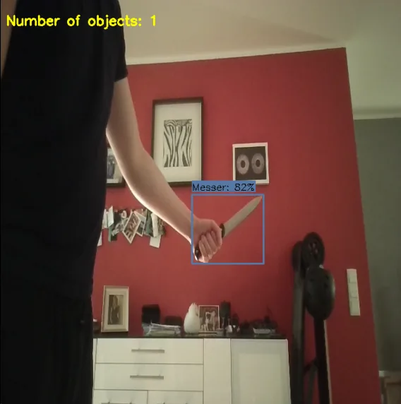
- Dataset
- 731 knife images · 4,011 without a knife
- Model
- YOLOv11-S · 640 × 640 · 150 epochs
- Validation
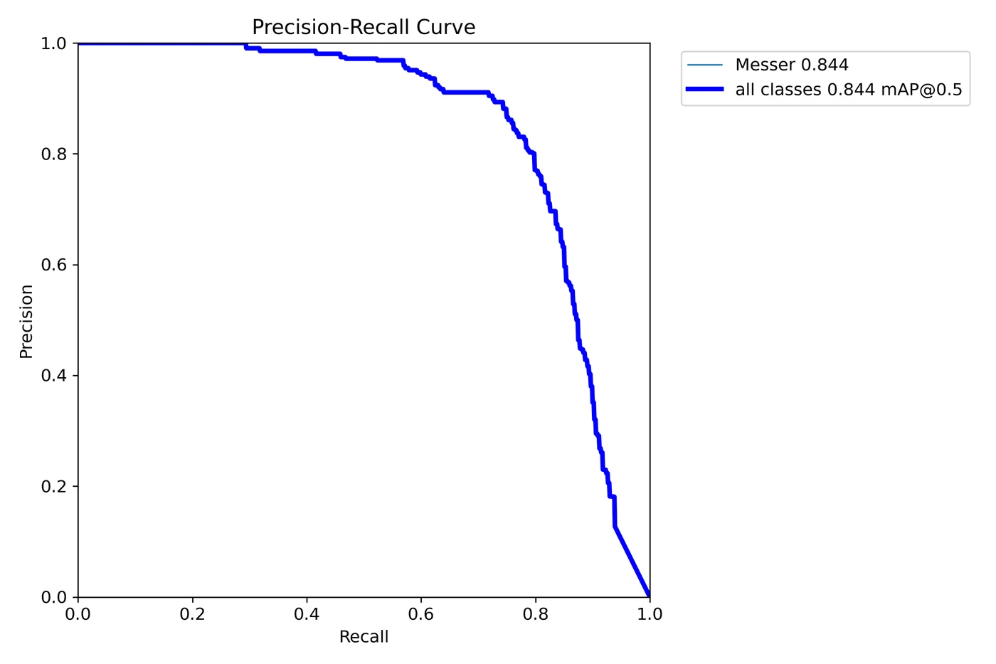
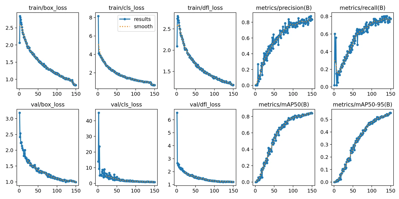
- mAP@0.5 = 0.844 · mAP@0.5:0.95 = 0.554
- Live performance
- 6–10 FPS observed on the laptop
Objective and ownership
The project explored early visual knife detection in live camera streams. I completed it independently over roughly 250 hours and started with very little prior computer-vision experience, learning Python, data labeling, YOLO training and edge deployment as the project progressed.
Self-recorded dataset
All images were recorded specifically for the project, including frames extracted from my own videos. The dataset contains 731 images with knives and 4,011 images without a knife, split into 3,781 training and 961 validation images — with 327 labeled boxes in the validation set. I reviewed the labels manually and later used auto-labeling to accelerate the process; total labeling effort was roughly 40–60 hours.
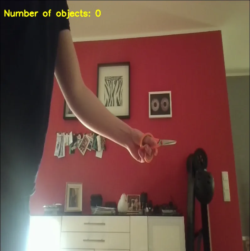
Early versions classified many hand-held objects as knives because the dataset did not contain enough representative negative scenes. Expanding the negative set to over 4,000 images removed the bulk of these false detections — the single most effective change in the project, and one that cost recording time rather than compute.
The class-structure experiment
An intermediate version split the label set into two classes: a knife lying in a scene, and a knife held in a hand. The reasoning was that the distinction carries the meaning for an alerting use case — an object on a counter is not the same event as an object in someone’s grip.
Measured against the merged single-class version on the same images and the same validation split, the split did not pay off. Every aggregate metric improved after collapsing the two classes back into one, and the standalone-knife class had been the weak half all along, with a small fraction of the instances of the held-knife class. Splitting a small dataset gave the model two under-supported problems instead of one well-supported one.
The comparison is not perfectly controlled — the merged run also trained for 150 instead of 110 epochs. But the direction is consistent across precision, recall and both mAP measures, and the single-class model is the one that ships.
| Metric | Two classes · 110 epochs | One class · 150 epochs |
|---|---|---|
| mAP@0.5 | 0.802 | 0.844 |
| mAP@0.5:0.95 | 0.516 | 0.554 |
| Precision | 0.812 | 0.841 |
| Recall | 0.739 | 0.768 |
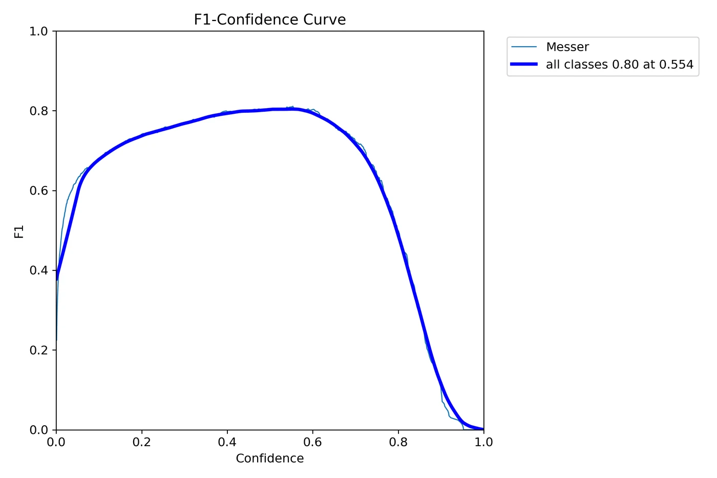
| Best F1 | 0.77 at conf. 0.502 | 0.80 at conf. 0.554 |
Training configuration
Rather than reporting a vague number of experiments, here is the exact configuration behind the shipping model. It ran in 2 hours 23 minutes on the Tesla T4 described further down.
| Parameter | Value |
|---|---|
| Base weights | yolo11s.pt (pretrained) |
| Classes | 1 — Messer |
| Input resolution | 640 × 640 |
| Epochs | 150 · best checkpoint at epoch 148 |
| Batch size | 16 |
| Optimizer | auto (SGD selected) · lr0 0.01 · lrf 0.01 · momentum 0.937 |
| Augmentation | mosaic 1.0 (closed for last 10 epochs) · fliplr 0.5 · HSV · scale 0.5 · erasing 0.4 |
| Seed | 0 · deterministic |
| Training time | 2 h 23 min on a single Tesla T4 |
Measured results
The following figures come from the validation set at the best checkpoint. They describe this dataset and this split — see the open points at the end of the page for what they do not yet prove.
| Metric | Value |
|---|---|
| mAP@0.5 | 0.844 |
| mAP@0.5:0.95 | 0.554 |
| Precision (best epoch) | 0.841 |
| Recall (best epoch) | 0.768 |
| Best F1 | 0.80 at confidence 0.554 |
| Precision reaches 1.00 | at confidence 0.862 |
| Maximum recall | 0.92 |
Where the model actually fails
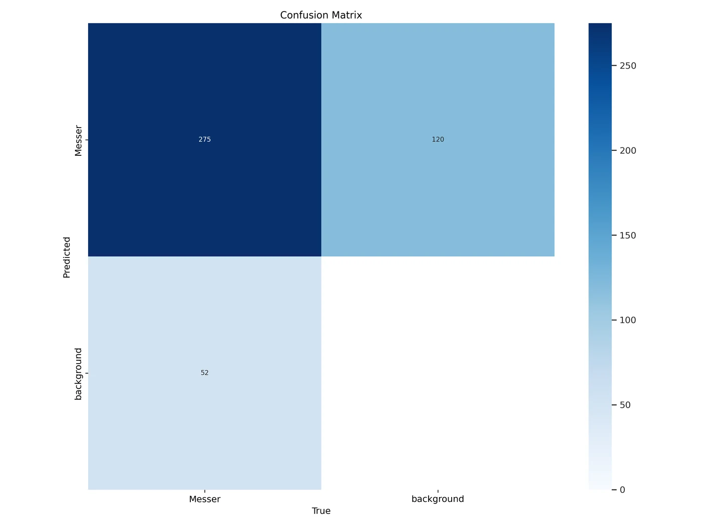
The aggregate numbers hide the more useful information, so here is the error structure from the confusion matrix at the default confidence threshold. Of 327 labeled instances in the validation set, 275 were detected and 52 were missed.
The bigger problem is the other direction: 120 detections landed on background regions containing no labeled object. That is roughly one false alarm for every 2.3 correct detections. The model over-triggers rather than under-triggers, and for an alerting application that is the more expensive failure mode. It is also the one number that barely moved between the two training runs, which tells me it is a property of the data rather than of the label structure — the next round has to target it with harder negative scenes.
- Detected: 275 of 327 labeled instances (84%)
- Missed: 52 instances (16%)
- False positives on background: 120
- Reliability drops with occlusion and unusual knife shapes
Live deployment
The model runs from a live webcam on a Lenovo Yoga Slim 6 at an observed 6–10 FPS, and on NVIDIA Jetson platforms including an Orin Nano Super. It was demonstrated in unfamiliar scenes across different lighting conditions and backgrounds.
Infrastructure: what the workstation really cost
In March 2025 I sourced almost all components second-hand and built a local AI workstation for approximately €910 instead of renting GPU time. Measured purely in compute, that decision does not pay off, and it is worth saying so plainly.
A T4-class cloud instance currently costs roughly $0.20 to $0.76 per hour on demand. At the middle of that range the €910 machine breaks even at about 3,300 GPU-hours — 137 days of continuous training. Across every run in this project I have used on the order of 100 hours. Renting that compute would have cost around €30. Per hour actually used, the workstation was roughly thirty times more expensive than renting.
Three things justified it anyway, and none of them is the hourly rate. First, the dataset is video recorded in my own home and shows me and my surroundings; uploading it to a third-party provider was not something I was willing to do. Second, a marginal cost of zero changed how I worked — the class-structure experiment above, the most useful result in this project, happened because one more training run cost nothing. Under metered billing I would have run fewer experiments and learned less. Third, €910 bought a complete workstation rather than GPU hours: the Ryzen 7 5800X, 64 GB of RAM and the 1 TB drive also carry CAD work and slicing, so charging the full amount to this project overstates it. Cloud GPU pricing was also considerably higher when I made the decision than it is today.
The honest conclusion is a rule rather than a verdict: for a project of this size without a data-protection constraint, renting is the correct choice at current prices, and I would rent. The purchase was justified by that constraint and by the value of unmetered iteration — not by the arithmetic.
| Position | Figure |
|---|---|
| Purchase price | ≈ €910, almost entirely second-hand, incl. a negotiated CPU/mainboard/RAM bundle |
| Core hardware | NVIDIA Tesla T4 · Ryzen 7 5800X · 64 GB RAM · 1 TB Samsung 990 Pro |
| Compute actually used | On the order of 100 GPU-hours across all runs |
| Same compute rented | ≈ €30 at $0.30 per hour |
| Break-even vs. renting | ≈ 3,300 GPU-hours, roughly 30× my actual usage |
| Energy | Training scheduled during local PV generation, after the 2 kWh battery was full |
What a real deployment would cost
A prototype answers "does it detect?". An operator asks "what does it cost to run?" — and my own false-positive rate answers that, because in an alerting system every false alarm consumes a person’s attention. The arithmetic below uses stated assumptions rather than a customer’s real figures, and it changed which engineering work I consider worth doing next.
Assumed scenario: one monitored entrance of a commercial building, four cameras, roughly 312 operating hours per month. One frame evaluated per second per camera, 30 seconds of human review per alarm, €20 per hour of fully loaded labour. Hardware at the prices I actually paid: €250 per Jetson Orin Nano Super plus an estimated €50 per camera module. Mounting, network and enclosures are not included.
Hardware is not the problem. Four nodes cost €1,200 once. Without any filtering, a 12.5 % false-positive rate per frame produces about 1,800 alarms per hour across four cameras — that is fifteen people occupied full time, which settles the question of whether the raw model is deployable. Requiring three consecutive detections before raising an alarm costs nothing in hardware and brings that to 28 alarms per hour, or roughly €1,460 per month in review time. The one-off hardware cost is overtaken by review labour in under a month.
The interesting consequence is non-linear. Because a three-frame filter raises the per-frame rate to the third power, halving the false-positive rate does not halve the review cost — it cuts it by a factor of eight, from about €1,460 to about €180 per month. That converts "improve the model somewhat" into a quantified return, and it puts the cheap lever ahead of the obvious one: filtering first at zero cost, then roughly 40 to 60 hours of additional negative-scene recording, and only then any question of a larger model.
- Capex: €1,200 once for four nodes, at the prices I paid
- Opex is dominated by human attention, not by hardware or energy
- Halving the false-positive rate returns roughly a factor of eight on review cost
- Cheapest effective lever is temporal filtering, which costs nothing to implement
| Consecutive detections required | Alarms per hour, 4 cameras | Review time | Review cost per month |
|---|---|---|---|
| 1 (no filter) | ≈ 1,800 | 15 people full time | not operable |
| 2 | ≈ 225 | 112 min per hour | ≈ €11,700 |
| 3 | ≈ 28 | 14 min per hour | ≈ €1,460 |
| 4 | ≈ 3.5 | 2 min per hour | ≈ €180 |
Result
The project produced a working live demonstration, a measured baseline of mAP@0.5 = 0.844, and reusable training hardware that still serves later projects. Its most transferable lesson was that data composition mattered more than model size or label sophistication: the decisive improvements came from recording thousands of the right negative scenes, and from simplifying the label structure rather than refining it. The model is YOLOv11-S — the small variant — and it is not the limiting factor.